Analysing the results of the constraint scan

import cobra
import matplotlib.pyplot as plt
import numpy as np
import pandas as pd
import seaborn as sns
from matplotlib.cm import ScalarMappable
from matplotlib.colors import Normalize
from matplotlib.ticker import AutoMinorLocator, MultipleLocator
from mmon_gcm.analysing import get_phase_lengths
from mmon_gcm.supermodel import SuperModel
from sklearn.linear_model import LinearRegression
from sklearn.metrics import mean_squared_error, r2_score
from sklearn.preprocessing import OneHotEncoder, StandardScaler

sns.set_theme()
sns.set_style("ticks")
palettes = {
    "tol_bright": sns.color_palette(
        ["#4477AA", "#66CCEE", "#228833", "#CCBB44", "#EE6677", "#AA3377", "#BBBBBB"]
    ),
    "tol_muted": sns.color_palette(
        [
            "#332288",
            "#88CCEE",
            "#44AA99",
            "#117733",
            "#999933",
            "#DDCC77",
            "#CC6677",
            "#882255",
            "#AA4499",
        ]
    ),
}
sns.set_palette(palettes["tol_muted"])

colours = sns.color_palette()

params = {
    "xtick.labelsize": "large",
    "ytick.labelsize": "large",
    "axes.labelsize": "large",
    "axes.titlesize": "x-large",
    "font.family": "sans-serif",
    "axes.spines.right": False,
    "axes.spines.top": False,
    "legend.frameon": False,
    "savefig.bbox": "tight",
    "lines.linewidth": 2.5,
    "figure.figsize": [5, 3.75],
    "figure.dpi": 150,
}
plt.rcParams.update(params)

def get_bounds_in_model(constraints):
    super_model = SuperModel(constraints)
    volumes = super_model.get_volumes(per_guard_cell=False)
    closed_volume = volumes[0]
    open_volume = volumes[1]
    osmolarities = super_model.get_osmolarities()
    closed_osmolarity = osmolarities[0]
    open_osmolarity = osmolarities[1]
    photons = super_model.get_photons(150)
    gc_photons = photons[0]
    gc_atpase_upper_bound = super_model.get_atpase_constraint_value(
        constraints.loc["ATPase"]
    )

    return {
        "V_closed": closed_volume,
        "V_open": open_volume,
        "Os_closed": closed_osmolarity,
        "Os_open": open_osmolarity,
        "Photons": gc_photons,
        "ATPase": gc_atpase_upper_bound,
    }

Importing results and constraints

# import results files
blue_results = pd.read_csv(
    "../outputs/constraint_scan/constraint_scan_results_blue.csv", index_col=0
)
white_results = pd.read_csv(
    "../outputs/constraint_scan/constraint_scan_results_white.csv", index_col=0
)
scan_results = pd.concat([white_results, blue_results])
scan_results = scan_results.reset_index().drop("index", axis=1)
# remove solutions which were not feasible
infeasible_solutions = scan_results[scan_results.isna().any(axis=1)]
feasible_solutions = scan_results.dropna()
scan_results = feasible_solutions

len(infeasible_solutions)

2

len(feasible_solutions)

1934

scan_results.shape

(1934, 7101)

# convert any fluxes that are below 10^-6 to 0
scan_results = scan_results.mask(abs(scan_results) < 0.000001, other=0)

# import constraints files
white_constraints = pd.read_csv(
    "../outputs/constraint_scan/constraints_df.csv", index_col=0
)
white_constraints["light"] = "white"
blue_constraints = pd.read_csv(
    "../outputs/constraint_scan/constraints_df.csv", index_col=0
)
blue_constraints["light"] = "blue"
scan_constraints = pd.concat([white_constraints, blue_constraints])
scan_constraints = scan_constraints.reset_index().drop("index", axis=1)
# remove infeasible constraints combinations
feasible_scan_constraints = scan_constraints.loc[feasible_solutions.index]
infeasible_scan_constraints = scan_constraints.loc[infeasible_solutions.index]
scan_constraints = feasible_scan_constraints

# Remove maintenance in scan_constraints
#scan_constraints = scan_constraints.drop('Maintenance', axis=1)

scan_constraints.columns

Index(['P_abs', 'T_l', 'A_l', 'V_gc_ind', 'FqFm', 'R_ch', 'R_ch_vol', 'L_air',
       'L_epidermis', 'Vac_frac', 'T', 'R', 'N_gcs', 'n', 'm', 'r', 's',
       'C_apo', 'A_closed', 'A_open', 'ATPase', 'light'],
      dtype='object')

# import constraints that were used in previous paper solutions
default_constraints = pd.read_csv("../inputs/arabidopsis_parameters.csv", index_col=0)[
    "Value"
]

paper_constraints = []
index = []
for light in ["white", "blue", "nops"]:
    for constraint in ["unconstrained", "constrained"]:
        constraints = default_constraints.copy()
        if constraint == "unconstrained":
            constraints["ATPase"] = 1000
        elif constraint == "constrained":
            constraints["ATPase"] = 7.48
        constraints["light"] = light
        index.append(f"{light}_{constraint}_wt")
        paper_constraints.append(constraints)
paper_constraints = pd.DataFrame(paper_constraints, index=index)
paper_constraints = paper_constraints.iloc[1, :-1]
paper_constraints

P_abs                  0.9
T_l                0.00017
A_l                    1.0
V_gc_ind               0.0
FqFm                   0.9
R_ch              0.069231
R_ch_vol          0.200476
L_air                 0.37
L_epidermis           0.15
Vac_frac             0.751
T                   296.15
R                  0.08205
N_gcs          580000000.0
n                      2.5
m                      0.8
r                      0.0
s                      0.0
C_apo              0.02302
A_closed               1.6
A_open                2.75
ATPase                7.48
Name: white_constrained_wt, dtype: object

# import results for previous simulations in paper
paper_solution_files = []

for light in ["white", "blue", "nops"]:
    for constraint in ["unconstrained", "constrained"]:
        paper_solution_files.append(f"{light}_{constraint}_wt.csv")
solution_dfs = [
    pd.read_csv(f"../outputs/model_solutions/{file_name}", index_col=0)["fluxes"]
    for file_name in paper_solution_files
]
paper_results = pd.concat(solution_dfs, axis=1).T
paper_results.index = index

# get a reduced get of constraints that are more specific to the guard cell

scan_gc_constraints = pd.DataFrame.from_dict(
    list(scan_constraints.apply(get_bounds_in_model, axis=1))
)
scan_gc_constraints["Os_dif"] = (
    scan_gc_constraints["Os_open"] - scan_gc_constraints["Os_closed"]
)
scan_gc_constraints.index = scan_constraints.index
scan_gc_constraints.head()

/home/maurice/Sync/GC/mmon-gcm/mmon_gcm/supermodel.py:23: UserWarning: No fba model added to the Supermodel, fine if that's what you want
  warnings.warn("No fba model added to the Supermodel, fine if that's what you want")

	V_closed	V_open	Os_closed	Os_open	Photons	ATPase	Os_dif
0	0.000157	0.000476	0.033212	0.278138	0.107908	0.004851	0.244926
1	0.000321	0.000738	0.067499	0.370715	0.106820	0.000585	0.303216
2	0.000248	0.000268	0.059662	0.070491	0.031490	0.004505	0.010828
3	0.000134	0.000278	0.033181	0.140030	0.013079	0.004855	0.106849
4	0.000438	0.000786	0.107888	0.313097	0.034626	0.011479	0.205209

paper_gc_constraints = pd.Series(get_bounds_in_model(paper_constraints))
paper_gc_constraints["Os_dif"] = (
    paper_gc_constraints["Os_open"] - paper_gc_constraints["Os_closed"]
)
paper_gc_constraints

/home/maurice/Sync/GC/mmon-gcm/mmon_gcm/supermodel.py:23: UserWarning: No fba model added to the Supermodel, fine if that's what you want
  warnings.warn("No fba model added to the Supermodel, fine if that's what you want")

V_closed     0.000220
V_open       0.000254
Os_closed    0.039359
Os_open      0.054922
Photons      0.018372
ATPase       0.004338
Os_dif       0.015563
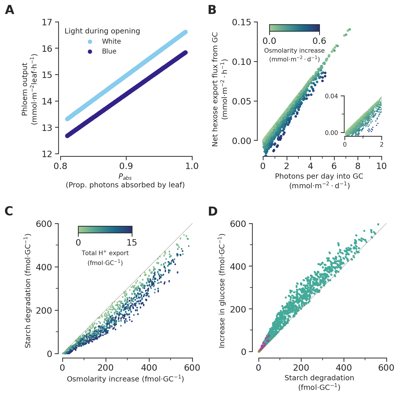
dtype: float64

7a - What contributes to phloem output?

Set up features for linear regression by

Convert light using onehotencoder

scan_constraints[["light"]]

	light
0	white
1	white
2	white
3	white
4	white
...	...
1931	blue
1932	blue
1933	blue
1934	blue
1935	blue

1934 rows × 1 columns

# extract the subject column as a pandas DataFrame
light = scan_constraints[["light"]]
# setting sparse=False means that enc.transform() will return an array
enc = OneHotEncoder(sparse_output=False)

# fit the encoder to the data
enc.fit(light)

# encode the data
light_enc = enc.transform(light)
light_columns = pd.DataFrame(light_enc, columns="light_" + enc.categories_[0], index=scan_constraints.index) # Added index=scan_constraints.index 
full_features = scan_constraints.drop("light", axis=1).join(light_columns)
gc_features = scan_gc_constraints.join(light_columns)

Also create scaled versions of features

scaler = StandardScaler()

scaler.fit(full_features)
full_features_scaled = scaler.transform(full_features)

scaler.fit(gc_features)
gc_features_scaled = scaler.transform(gc_features)

full_features[full_features.isna().any(axis=1)]

	P_abs	T_l	A_l	V_gc_ind	FqFm	R_ch	R_ch_vol	L_air	L_epidermis	Vac_frac	...	n	m	r	s	C_apo	A_closed	A_open	ATPase	light_blue	light_white

0 rows × 23 columns

Compare full and gc features

response = scan_results.Phloem_tx_overall
#response = scan_results.Photon_tx_gc_3

lm_full = LinearRegression()
lm_full.fit(full_features, response)
full_pred = lm_full.predict(full_features)
print("Mean squared error, MSE = %.5f" % mean_squared_error(response, full_pred))
print("Coefficient of determination, r2 = %.5f" % r2_score(response, full_pred))

lm_gc = LinearRegression()
lm_gc.fit(gc_features, response)
gc_pred = lm_gc.predict(gc_features)
print("Mean squared error, MSE = %.5f" % mean_squared_error(response, gc_pred))
print("Coefficient of determination, r2 = %.5f" % r2_score(response, gc_pred))

Mean squared error, MSE = 0.00040
Coefficient of determination, r2 = 0.99960
Mean squared error, MSE = 0.87829
Coefficient of determination, r2 = 0.12388

So can’t predict phloem output using GC features, but can predict pretty well using the full set

Which features are most important?

pd.DataFrame(lm_full.coef_, index=full_features.columns).sort_values(by=0)

	0
T_l	-4.514050e-01
light_blue	-3.533915e-01
C_apo	-1.320172e-03
m	-8.770751e-04
Vac_frac	-7.229537e-04
A_open	-2.302990e-04
FqFm	-6.018903e-05
n	-5.320860e-05
V_gc_ind	-9.982424e-10
r	-6.477489e-12
N_gcs	-1.186773e-12
A_l	-2.997951e-13
R	-1.131064e-13
s	1.957373e-11
T	4.679942e-06
ATPase	4.859983e-06
A_closed	1.710221e-04
L_epidermis	2.027958e-04
L_air	2.972018e-04
R_ch_vol	4.995322e-04
R_ch	1.383114e-03
light_white	3.533915e-01
P_abs	1.800514e+01

Lots of unimportant features so we can use lasso regression to see which ones we really need

Try different alphas for lasso to see r2

from sklearn.linear_model import Lasso

alphas = np.linspace(0.01, 0.1, 10)
r2s = []

for alpha in alphas:
    lasso = Lasso(alpha=alpha)
    lasso.fit(full_features, response)
    lasso_pred = lasso.predict(full_features)
    r2s.append(r2_score(response, lasso_pred))

pd.Series(r2s, index=alphas)

0.01    0.962288
0.02    0.850360
0.03    0.663812
0.04    0.402646
0.05    0.116440
0.06    0.111850
0.07    0.106593
0.08    0.100528
0.09    0.093654
0.10    0.085972
dtype: float64

from sklearn.linear_model import Lasso

alphas = np.linspace(0.001, 0.01, 10)
r2s = []

for alpha in alphas:
    lasso = Lasso(alpha=alpha)
    lasso.fit(full_features, response)
    lasso_pred = lasso.predict(full_features)
    r2s.append(r2_score(response, lasso_pred))

pd.Series(r2s, index=alphas)

0.001    0.999224
0.002    0.998105
0.003    0.996240
0.004    0.993628
0.005    0.990270
0.006    0.986166
0.007    0.981316
0.008    0.975719
0.009    0.969377
0.010    0.962288
dtype: float64

Lets take 0.03 as it’s highest that rounds to 0.999

Lasso with alpha = 0.003

lasso = Lasso(alpha=0.003)
lasso.fit(full_features, response)
lasso_pred = lasso.predict(full_features)
lass_coefs = pd.DataFrame(lasso.coef_, index=full_features.columns).sort_values(by=0)
# display coefficients that aren't 0
lass_coefs[abs(lass_coefs.loc[:, 0]) > 0.00001]

	0
light_blue	-0.694783
T	-0.000436
A_open	-0.000309
P_abs	16.894629

P_abs and light are by far the largest coefficients

Try scaled as well

from sklearn.linear_model import Lasso

alphas = np.linspace(0.01, 0.1, 10)
r2s = []

for alpha in alphas:
    lasso = Lasso(alpha=alpha)
    lasso.fit(full_features_scaled, response)
    lasso_pred = lasso.predict(full_features_scaled)
    r2s.append(r2_score(response, lasso_pred))

pd.Series(r2s, index=alphas)

0.01    0.999398
0.02    0.998799
0.03    0.997801
0.04    0.996405
0.05    0.994609
0.06    0.992415
0.07    0.989821
0.08    0.986829
0.09    0.983437
0.10    0.979646
dtype: float64

lasso = Lasso(alpha=0.01)
lasso.fit(full_features_scaled, response)
lasso_pred = lasso.predict(full_features_scaled)
lass_coefs = pd.DataFrame(lasso.coef_, index=full_features.columns).sort_values(by=0)
print(f"r2 score: {r2_score(response, lasso_pred)}")
# display coefficients that aren't 0
lass_coefs[abs(lass_coefs.loc[:, 0]) > 0.00001]

r2 score: 0.9993975321339854

	0
light_blue	-0.343392
P_abs	0.926581

When scaled this is even clearer

def phloemoutput_subfig(ax):
    for light, colour in zip(
        ["white", "blue"], [sns.color_palette()[1], sns.color_palette()[0]]
    ):
        constraints_light_df = scan_constraints[scan_constraints.light == light]
        results_light_df = scan_results[scan_constraints.light == light]

        ax.scatter(
            constraints_light_df.P_abs,
            results_light_df.Phloem_tx_overall,
            label=light.capitalize(),
            color=colour,
        )

    ax.legend(title="Light during opening", loc="upper left")  # Set loc to "upper left"
    ax.set_xlabel("$P_{abs}$\n(Prop. photons absorbed by leaf)", size="medium")
    ax.set_ylabel(
        "Phloem output\n(mmol$\cdot$m$^{-2}$leaf$\cdot$h$^{-1}$)", size="medium"
    )

    ax.set_ylim(11.9, 17)
    ax.set_xlim(0.797, 1)
    ax.spines["left"].set_bounds(12, 17)
    ax.spines["bottom"].set_bounds(0.8, 1)
    ax.xaxis.set_major_locator(MultipleLocator(0.1))
    # ax.xaxis.set_minor_locator(AutoMinorLocator(2))
    ax.yaxis.set_major_locator(MultipleLocator(1))
    # ax.yaxis.set_minor_locator(AutoMinorLocator(2))

    ax.set_aspect(abs(1 - 0.8) / abs(17 - 12))

    return ax


fig, ax = plt.subplots()
phloemoutput_subfig(ax)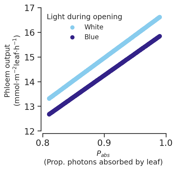

7b - What affects hexose export from the guard cell?

Generate hexose export df

four_stage_GC_model = cobra.io.sbml.read_sbml_model(
    "../models/4_stage_GC.xml"
)  # read model

# get total flux across all phases
net_carbon_dict = {}
for metabolite in ["GLC", "FRU", "SUCROSE"]:
    net_metabolite = 0
    for i, phase_length in enumerate(get_phase_lengths(four_stage_GC_model)):
        phase_number = i + 1
        net_metabolite = (
            net_metabolite
            + scan_results.loc[:, f"{metabolite}_ae_gc_{phase_number}"] * phase_length
        )
    net_carbon_dict[metabolite] = net_metabolite
net_carbon_df = pd.DataFrame.from_dict(net_carbon_dict)

# correct for fact that sucrose is two hexoses
net_carbon = (
    net_carbon_df.GLC + net_carbon_df.FRU + net_carbon_df.SUCROSE * 2
) * -1  # mmol.m2-1
net_carbon = net_carbon * 10**-3  # moles.m2-1
carbon_per_gc = net_carbon / scan_constraints.N_gcs  # moles.gc-1
carbon_per_gc = carbon_per_gc * 10**15  # fmol.gc-1

No objective coefficients in model. Unclear what should be optimized

Fit model to hexose export

response = carbon_per_gc
for features in [full_features, gc_features]:
    lm_1 = LinearRegression()
    lm_1.fit(features, response)
    pred = lm_1.predict(features)
    print("Mean squared error, MSE = %.2f" % mean_squared_error(response, pred))
    print("Coefficient of determination, r2 = %.2f" % r2_score(response, pred))

Mean squared error, MSE = 392.25
Coefficient of determination, r2 = 0.45
Mean squared error, MSE = 118.22
Coefficient of determination, r2 = 0.83

So hexose export can be better predicted using the gc features compared to all the features. Is this because it’s hexose per gc?

response = net_carbon
for features in [full_features, gc_features]:
    lm_1 = LinearRegression()
    lm_1.fit(features, response)
    pred = lm_1.predict(features)
    print("Mean squared error, MSE = %.2f" % mean_squared_error(response, pred))
    print("Coefficient of determination, r2 = %.2f" % r2_score(response, pred))

Mean squared error, MSE = 0.00
Coefficient of determination, r2 = 0.52
Mean squared error, MSE = 0.00
Coefficient of determination, r2 = 1.00

Seems so, as we’re confusing things by introducing the N_gcs division into the response

response = net_carbon
lm_1 = LinearRegression()
lm_1.fit(gc_features, response)
pred = lm_1.predict(gc_features)
lm_coefs = pd.DataFrame(lm_1.coef_, index=gc_features.columns).sort_values(by=0)
lm_coefs[abs(lm_coefs.loc[:, 0]) > 0.00001]

	0
light_blue	-1.381741e+08
light_white	-1.381741e+08
Os_open	-8.054295e+05
V_closed	-1.611919e-02
ATPase	1.462491e-04
Photons	2.354302e-04
V_open	6.360736e-03
Os_dif	8.054295e+05
Os_closed	8.054295e+05

Mainly different light colours as well as osmolarity. What if we correct for light colour?

Create a reponse for total photons into the GC, irrespective of blue or white light

photon_influx = scan_results.loc[:, "Photon_tx_gc_3"]
photon_hours = scan_constraints.loc[:, "light"].apply(
    lambda x: 12 if x == "white" else 11.5
)
total_photons_per_day = photon_influx * photon_hours

response = net_carbon
features = np.array([total_photons_per_day]).T
lm_1 = LinearRegression()
lm_1.fit(features, response)
pred = lm_1.predict(features)
print("Mean squared error, MSE = %.6f" % mean_squared_error(response, pred))
print("Coefficient of determination, r2 = %.6f" % r2_score(response, pred))
pd.DataFrame(lm_1.coef_, index=["Photons per day"]).sort_values(by=0)

Mean squared error, MSE = 0.000000
Coefficient of determination, r2 = 0.952128

	0
Photons per day	0.000019

response = net_carbon
features = np.array([total_photons_per_day, gc_features.Os_dif]).T
lm_1 = LinearRegression()
lm_1.fit(features, response)
pred = lm_1.predict(features)
print("Mean squared error, MSE = %.6f" % mean_squared_error(response, pred))
print("Coefficient of determination, r2 = %.6f" % r2_score(response, pred))
pd.DataFrame(lm_1.coef_, index=["Photons per day", "Os dif"]).sort_values(by=0)

Mean squared error, MSE = 0.000000
Coefficient of determination, r2 = 0.997839

	0
Os dif	-0.000042
Photons per day	0.000020

Pretty good R2

response = net_carbon
features = np.array(gc_features.ATPase).reshape(-1, 1)
lm_1 = LinearRegression()
lm_1.fit(features, response)
pred = lm_1.predict(features)
print("Mean squared error, MSE = %.6f" % mean_squared_error(response, pred))
print("Coefficient of determination, r2 = %.6f" % r2_score(response, pred))
pd.DataFrame(lm_1.coef_, index=["ATPase"]).sort_values(by=0)

Mean squared error, MSE = 0.000000
Coefficient of determination, r2 = 0.109253

	0
ATPase	0.001702

ATPase can’t really predict hexose export, at least not by itself

def photons_vs_carbon_export_subfig(ax):
    max_os_dif = scan_gc_constraints.Os_dif.max().round(1)
    norm = Normalize(vmin=0, vmax=max_os_dif)
    mappable = ScalarMappable(norm=norm, cmap=sns.color_palette("crest", as_cmap=True))

    net_carbon_mmol = net_carbon * 10**3

    ax.scatter(
        total_photons_per_day,
        net_carbon_mmol,
        c=scan_gc_constraints.Os_dif,
        norm=norm,
        s=10,
        cmap=sns.color_palette("crest", as_cmap=True),
    )

    cbaxes = ax.inset_axes([0.1, 0.93, 0.40, 0.05])
    cbar = plt.colorbar(
        mappable, cax=cbaxes, ticks=[0, max_os_dif], orientation="horizontal"
    )
    cbar.set_label("Osmolarity increase\n(mmol$\cdot$m$^{-2}\cdot$d$^{-1}$)", size=10)

    inset_ax = ax.inset_axes([0.7, 0.15, 0.3, 0.3])
    inset_ax.scatter(
        total_photons_per_day,
        net_carbon_mmol,
        c=scan_gc_constraints.Os_dif,
        s=1,
        cmap=sns.color_palette("crest", as_cmap=True),
    )
    inset_ax.set_xlim([-0.3 / 10, 2])
    inset_ax.set_ylim([-0.02 / 5, 0.04])
    inset_ax.tick_params(labelsize=10)
    inset_ax.spines["left"].set_bounds(0, 0.04)
    inset_ax.spines["bottom"].set_bounds(0, 2)
    inset_ax.yaxis.set_major_locator(MultipleLocator(0.04))
    inset_ax.yaxis.set_minor_locator(AutoMinorLocator(2))
    inset_ax.xaxis.set_major_locator(MultipleLocator(2))
    inset_ax.xaxis.set_minor_locator(AutoMinorLocator(2))

    ax.set_xlim([-0.5, 10])
    ax.set_ylim([-0.02, 0.15])
    ax.spines["left"].set_bounds(0, 0.15)
    ax.spines["bottom"].set_bounds(0, 10)
    ax.xaxis.set_major_locator(MultipleLocator(2))
    ax.xaxis.set_minor_locator(AutoMinorLocator(2))
    ax.yaxis.set_major_locator(MultipleLocator(0.05))
    ax.set_aspect(abs(10 - 0) / abs(0.15 - 0))

    ax.set_xlabel(
        "Photons per day into GC\n" + r"(mmol$\cdot$m$^{-2}\cdot$d$^{-1}$)",
        size="medium",
    )
    ax.set_ylabel(
        "Net hexose export flux from GC\n" + r"(mmol$\cdot$m$^{-2}\cdot$h$^{-1}$)",
        size="medium",
    )

    return ax


fig, ax = plt.subplots()
photons_vs_carbon_export_subfig(ax)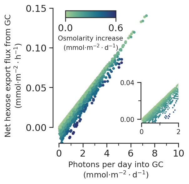

Are there any solutions where net carbon export are below 0?

(net_carbon < 0).sum()

177

(net_carbon > 0).sum()

1757

(net_carbon == 0).sum()

0

1-((net_carbon < 0).sum())/len(net_carbon)

0.9084798345398138

What’s interesting about them?

scan_constraints.loc[net_carbon < 0]

	P_abs	T_l	A_l	V_gc_ind	FqFm	R_ch	R_ch_vol	L_air	L_epidermis	Vac_frac	...	N_gcs	n	m	r	s	C_apo	A_closed	A_open	ATPase	light
3	0.880998	0.000192	1.0	8.629192e-13	0.866582	0.051244	0.204472	0.309538	0.169957	0.813726	...	3.851195e+08	2.077401	0.940848	5.747590e-14	1.515328e-13	0.029770	3.399462	9.936390	12.606738	white
30	0.977490	0.000213	1.0	8.097892e-13	0.849340	0.085944	0.200220	0.228127	0.106448	0.830654	...	6.380687e+08	2.318837	0.830687	7.864234e-14	1.643929e-13	0.025288	3.333199	10.672109	11.311688	white
35	0.856504	0.000237	1.0	1.360312e-12	0.860652	0.067374	0.192203	0.258071	0.107286	0.777399	...	8.423951e+08	2.039681	0.993173	6.491681e-14	2.153582e-13	0.029056	3.839122	9.599664	13.331786	white
45	0.930783	0.000189	1.0	1.489148e-12	0.888709	0.046345	0.194218	0.231172	0.183409	0.831117	...	1.105337e+09	2.328963	0.866898	6.554262e-14	2.276119e-13	0.023463	3.689994	11.705067	7.102036	white
64	0.859688	0.000235	1.0	3.426082e-12	0.791894	0.052688	0.198979	0.230128	0.197351	0.842065	...	3.647771e+08	1.730236	0.919254	7.408027e-14	2.148666e-13	0.029782	1.697687	11.305181	13.115608	white
...	...	...	...	...	...	...	...	...	...	...	...	...	...	...	...	...	...	...	...	...	...
1882	0.845869	0.000172	1.0	1.048237e-12	0.845831	0.080705	0.199110	0.334855	0.163015	0.764383	...	2.061369e+08	1.615056	0.959637	7.543702e-14	2.598267e-13	0.027358	1.738303	9.792686	12.376386	blue
1910	0.891865	0.000236	1.0	1.587349e-12	0.841325	0.047596	0.190368	0.187888	0.114146	0.818767	...	8.062927e+08	1.649409	0.853218	7.850763e-14	2.357539e-13	0.024782	1.406129	6.738719	13.099119	blue
1917	0.917349	0.000172	1.0	6.231750e-13	0.847565	0.047245	0.195349	0.244040	0.192836	0.789315	...	9.777013e+08	1.535770	0.824097	5.226121e-14	2.318500e-13	0.024413	1.599696	9.447559	0.599285	blue
1918	0.979824	0.000215	1.0	7.663475e-13	0.834459	0.092777	0.203782	0.191754	0.104075	0.832115	...	2.886042e+08	2.043540	0.833630	5.487253e-14	1.306311e-13	0.031694	1.449804	8.414919	3.970192	blue
1926	0.884257	0.000212	1.0	9.887656e-13	0.794346	0.042550	0.190401	0.318149	0.216369	0.817676	...	5.898101e+08	2.199278	0.968034	6.179313e-14	2.376930e-13	0.028122	2.487448	9.333051	11.542919	blue

177 rows × 22 columns

scan_gc_constraints.loc[net_carbon < 0]

	V_closed	V_open	Os_closed	Os_open	Photons	ATPase	Os_dif
3	0.000134	0.000278	0.033181	0.140030	0.013079	0.004855	0.106849
30	0.000272	0.000640	0.063820	0.310722	0.027134	0.007218	0.246902
35	0.000391	0.000706	0.109738	0.371630	0.037644	0.011231	0.261892
45	0.000519	0.001100	0.133538	0.606216	0.055639	0.007850	0.472678
64	0.000124	0.000384	0.020705	0.204952	0.033219	0.004784	0.184247
...	...	...	...	...	...	...	...
1882	0.000081	0.000206	0.013085	0.098841	0.013994	0.002551	0.085757
1910	0.000279	0.000617	0.040490	0.207920	0.027690	0.010562	0.167430
1917	0.000308	0.000709	0.044057	0.291729	0.022555	0.000586	0.247672
1918	0.000061	0.000171	0.010122	0.069783	0.011858	0.001146	0.059661
1926	0.000231	0.000480	0.050001	0.234255	0.015845	0.006808	0.184254

177 rows × 7 columns

Ok they are the same just with different light colours. Is it the photon/od_dif ratio?

scan_gc_constraints.loc[180, "Photons"] / scan_gc_constraints.loc[180, "Os_dif"]

0.8286998886406594

(scan_gc_constraints.loc[:, "Photons"] / scan_gc_constraints.loc[:, "Os_dif"]).min()

0.028310817388733575

Yes, it has the lowest photon:od_diff ratio of any combination

At our predicted level of osmolarity and other guard cell parameters, what would FqFm.R_ch need to be for guard cell to act as a sink?

\(e = FqFm \cdot R_{ch} \cdot R_{ch_{vol}}\) <- We want to know e, that is the capacity of guard cell vs mesophyll. Function of efficiency, number of chloroplasts, and valume of chloroplasts

\(P_{gc} = e \cdot v\_prop_{gc} \cdot P\)

\(e = \frac{P_{gc}}{v\_prop_{gc} \cdot P}\)

P = 150 * paper_constraints.P_abs
P = P * 10**-3 * 60 * 60  # umolessec-1 -> mmolhr-1

V_l = (
    paper_constraints.T_l * paper_constraints.A_l
)  # volume of leaf is area x thickness
V_l = V_l * 10**3  # (Total leaf volume) m3 -> dm3 = 10**3

V_gc = (
    paper_constraints.V_gc_ind * paper_constraints.N_gcs
)  # total volume of gc in leaf

# volume of meosphyll is leaf that isn't epidermis or air
V_me = V_l * (1 - paper_constraints.L_epidermis) * (1 - paper_constraints.L_air)

v_prop_gc = V_gc / V_me  # volume of gc is negligable

response = net_carbon
features = np.array([total_photons_per_day, gc_features.Os_dif]).T
lm_1 = LinearRegression()
lm_1.fit(features, response)
pred = lm_1.predict(features)
print("Mean squared error, MSE = %.6f" % mean_squared_error(response, pred))
print("Coefficient of determination, r2 = %.6f" % r2_score(response, pred))
print(f"Intercept: {lm_1.intercept_}")
pd.DataFrame(lm_1.coef_, index=["Photons per day", "Os dif"]).sort_values(by=0)

Mean squared error, MSE = 0.000000
Coefficient of determination, r2 = 0.997839
Intercept: -2.9943170116709816e-07

	0
Os dif	-0.000042
Photons per day	0.000020

$ C_{net} = -3^{-5}Os_{dif} + 2^{-5}P_{day} - 6.80 ^{-8}$

$ 0 = -3^{-5} + 2^{-5}P_{day} - 6.80 ^{-8}$

$ = P_{day}$

os_dif_coef = lm_1.coef_[1]
photons_per_day_coef = lm_1.coef_[0]
os_in_selected_scenarios = paper_gc_constraints.Os_dif
intercept = lm_1.intercept_

photons_needed = (
    intercept - os_dif_coef * os_in_selected_scenarios
) / photons_per_day_coef
photons_needed

0.01766160051488187

total_photons_per_day.min() / photons_needed

2.1088116678656323

So at that osmolarity for the guard cell to act as sink tissue the total level of photons coming in would have to be 15x lower than we see in any of our scenarios, which will be for blue light

photon_influx = photons_needed / 11.5

\(e = \frac{P_{gc}}{v\_prop_{gc} \cdot P}\)

e = photon_influx / (v_prop_gc * P)
e * 100

0.10441977210694658

So the capacity for photosynthesis in the guard cell only needs to be 0.1% of that of the mesophyll to act as a source tissue

What is the range of photosynthetic capacities that we use?

capacity_percentages = (scan_constraints.FqFm * scan_constraints.R_ch) * 100
print(f"High: {capacity_percentages.max()}")
print(f"Low: {capacity_percentages.min()}")

High: 16.086936580407595
Low: 2.773358075436272

7c - So does the ATPase have an effect on starch if not on hexose export very much?

How many solutions utilise starch?

starch = scan_results.STARCH_p_gc_Linker_1 - scan_results.STARCH_p_gc_Linker_2
print(f"{(starch > 0).sum()} or {(starch > 0).sum()/len(starch) * 100:.0f}%")

1892 or 98%

In how many of those solutions is the ATPase constrained?

atpase_constrained = (
    abs(scan_gc_constraints.ATPase - scan_results.PROTON_ATPase_c_gc_2) < 0.000001
)
(atpase_constrained & starch > 0).sum()

1864

((scan_gc_constraints.ATPase - scan_results.PROTON_ATPase_c_gc_2) < 0.000001).sum() / (starch > 0).sum()

0.985200845665962

(starch <= 0).sum()

42

scan_gc_constraints[(atpase_constrained & (starch == 0))]

	V_closed	V_open	Os_closed	Os_open	Photons	ATPase	Os_dif

So there is one solution which doesn’t

scan_gc_constraints[(atpase_constrained & starch < 0)]

	V_closed	V_open	Os_closed	Os_open	Photons	ATPase	Os_dif

#(scan_gc_constraints.loc[1685] - scan_gc_constraints.mean()) / scan_gc_constraints.std()

High photons, high ATPase, low osmolarity dif

How many constrained solutions don’t use starch?

(atpase_constrained & (starch == 0)).sum()

0

scan_gc_constraints[(atpase_constrained & (starch == 0))]

	V_closed	V_open	Os_closed	Os_open	Photons	ATPase	Os_dif

#(scan_gc_constraints.loc[1779] - scan_gc_constraints.mean()) / scan_gc_constraints.std()

Osmolarity difference is low, photons are high, atpase is low. Closed osmolarity is high, forcing the use of something else?

Increase per GC allows comparison with literature values

starch_per_gc = starch * 10**-3 / scan_constraints.N_gcs * 10**15  # fmol.gc-1

horrer_starch_level = 184

os_increase_per_gc = (
    scan_gc_constraints.Os_dif * 10**-3 / scan_constraints.N_gcs * 10**15
)
protons_moved_per_gc = (
    scan_results.PROTON_ATPase_c_gc_2 * 10**-3 / scan_constraints.N_gcs * 10**15
)

protons_moved_per_gc.max()

16.983568453252616

def starch_vs_os_subfig(ax):
    dot_size = 2

    norm = Normalize(vmin=0, vmax=15)
    mappable = ScalarMappable(norm=norm, cmap=sns.color_palette("crest", as_cmap=True))

    ax.plot([0, 600], [0, 600], c="grey", alpha=0.5, clip_on=False, linewidth=1)

    sc = ax.scatter(
        os_increase_per_gc,
        starch_per_gc,
        s=dot_size,
        c=protons_moved_per_gc,
        norm=norm,
        cmap=sns.color_palette("crest", as_cmap=True),
    )

    cbaxes = ax.inset_axes([0.15, 0.93, 0.40, 0.05])
    cbar = plt.colorbar(mappable, cax=cbaxes, ticks=[0, 15], orientation="horizontal")
    cbar.set_label("Total H$^{+}$ export\n(fmol$\cdot$GC$^{-1}$)", size=10)

    y_max = 600
    y_min = -20
    x_max = 600
    x_min = -20
    ax.set_ylim(y_min, y_max)
    ax.set_xlim(x_min, x_max)
    ax.spines["left"].set_bounds(0, y_max)
    ax.spines["bottom"].set_bounds(0, x_max)
    ax.xaxis.set_major_locator(MultipleLocator(200))
    ax.xaxis.set_minor_locator(AutoMinorLocator(2))
    ax.yaxis.set_major_locator(MultipleLocator(200))
    ax.yaxis.set_minor_locator(AutoMinorLocator(2))
    ax.set_aspect(1)

    ax.set_xlabel("Osmolarity increase (fmol$\cdot$GC$^{-1}$)", size="medium")
    ax.set_ylabel(r"Starch degradation (fmol$\cdot$GC$^{-1}$)", size="medium")
    # ax.hlines(-155, xmin=0.15, xmax=0.99, clip_on=False, linewidth=1, color='.15')

#     ax.hlines(
#         184,
#         xmin=0,
#         xmax=x_max,
#         linewidth=1,
#         linestyle="--",
#         color=sns.color_palette()[6],
#     )
#     ax.text(
#         x_max,
#         175,
#         "Horrer et al. (2016)",
#         ha="right",
#         va="top",
#         size="x-small",
#         color=sns.color_palette()[6],
#     )

#     paper_scenarios_colour = sns.color_palette()[2]
#     ax.vlines(
#         26.83,
#         ymin=0,
#         ymax=110,
#         linewidth=1,
#         linestyle="--",
#         color=paper_scenarios_colour,
#     )
#     ax.text(
#         50,
#         120,
#         "Paper\nscenarios",
#         ha="center",
#         va="bottom",
#         size="x-small",
#         color=paper_scenarios_colour,
#     )

    return ax


fig, ax = plt.subplots(figsize=(6, 4))

starch_vs_os_subfig(ax)

fig.savefig("../outputs/constraint_scan/atpase_vs_starch.svg")
fig.savefig("../outputs/constraint_scan/atpase_vs_starch.png")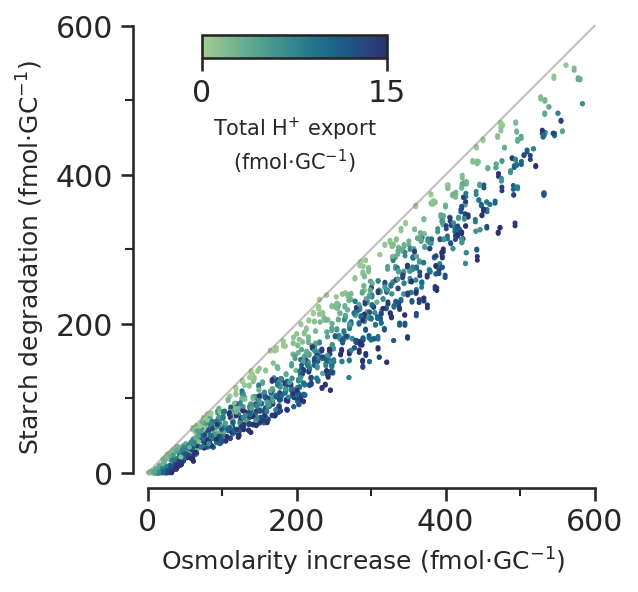

How do starch levels vary with white/blue light?

starch_per_gc

0       452.289024
1       277.547788
2         4.237398
3       167.427081
4        88.409571
           ...    
1931    401.554966
1932    111.326430
1933    269.642074
1934     81.257996
1935    271.281498
Length: 1934, dtype: float64

How is starch used?

What proportion of white light solutions that degrade starch use it for osmoticum?

(
    (
        (scan_constraints["light"] == "white")
        & (starch > 0)
        & (scan_results.RXN_2141_p_gc_2 > 0)
    ).sum()
) / ((scan_constraints["light"] == "white") & (starch > 0)).sum() * 100

100.0

What proportion of white light solutions that degrade starch use it for energy?

(
    (
        (scan_constraints["light"] == "white")
        & (starch > 0)
        & (scan_results.MALTODEG_RXN_c_gc_2 > 0)
    ).sum()
) / ((scan_constraints["light"] == "white") & (starch > 0)).sum() * 100

37.379162191192265

In the solutions that use it for energy, what is the average % used for energy?

(
    (
        (
            scan_results[
                (
                    (
                        (scan_constraints["light"] == "white")
                        & (starch > 0)
                        & (scan_results.MALTODEG_RXN_c_gc_2 > 0)
                    )
                )
            ].MALTODEG_RXN_c_gc_2
        )
        / starch[
            (
                (scan_constraints["light"] == "white")
                & (starch > 0)
                & (scan_results.MALTODEG_RXN_c_gc_2 > 0)
            )
        ]
    )
    * 100
).mean()

3.390568533696099

What proportion of blue light solutions that degrade starch use it for osmoticum?

(
    (
        (scan_constraints["light"] == "blue")
        & (starch > 0)
        & (scan_results.RXN_2141_p_gc_2 > 0)
    ).sum()
) / ((scan_constraints["light"] == "blue") & (starch > 0)).sum() * 100

96.98231009365244

((scan_constraints["light"] == "blue") & (starch > 0)).sum() - (
    (
        (scan_constraints["light"] == "blue")
        & (starch > 0)
        & (scan_results.RXN_2141_p_gc_2 > 0)
    ).sum()
)

29

29 solutions doesn’t

scan_constraints[
    (
        (scan_constraints["light"] == "blue")
        & (starch > 0)
        & ~(scan_results.RXN_2141_p_gc_2 > 0)
    )
]

	P_abs	T_l	A_l	V_gc_ind	FqFm	R_ch	R_ch_vol	L_air	L_epidermis	Vac_frac	...	N_gcs	n	m	r	s	C_apo	A_closed	A_open	ATPase	light
1017	0.982189	0.000231	1.0	1.217851e-12	0.806859	0.073278	0.211816	0.312352	0.170798	0.850346	...	7.505322e+08	2.216148	0.988893	7.629564e-14	2.378212e-13	0.036241	3.213625	3.269583	5.188912	blue
1029	0.987023	0.000221	1.0	1.629365e-12	0.838141	0.096801	0.204151	0.251819	0.217884	0.765830	...	3.634520e+08	1.950142	0.846086	7.725629e-14	1.043478e-13	0.028292	2.862462	3.198156	13.387886	blue
1056	0.833108	0.000195	1.0	1.641114e-12	0.848315	0.162755	0.206171	0.278300	0.189228	0.863030	...	4.977284e+08	1.533894	0.896850	7.795038e-14	1.909829e-13	0.034884	3.554507	3.763593	14.205187	blue
1101	0.986662	0.000234	1.0	4.080272e-12	0.833938	0.038088	0.195959	0.208027	0.195915	0.851504	...	1.080920e+09	2.176108	0.871806	6.374026e-14	1.607315e-13	0.031215	2.021054	2.957040	13.642663	blue
1175	0.845082	0.000195	1.0	3.099346e-12	0.858672	0.105619	0.192160	0.271365	0.122900	0.805677	...	1.156622e+09	1.676400	0.938192	7.393047e-14	1.742883e-13	0.034981	3.772808	3.898576	11.481076	blue
1210	0.979145	0.000175	1.0	5.704240e-13	0.888548	0.072428	0.191789	0.325010	0.203983	0.860514	...	1.036523e+09	1.899936	0.859060	5.463702e-14	1.576704e-13	0.028699	3.722164	4.071019	8.231288	blue
1241	0.964159	0.000240	1.0	3.888226e-12	0.849131	0.040710	0.202661	0.308670	0.218431	0.872428	...	3.693487e+08	2.243153	0.842068	6.859716e-14	2.559610e-13	0.035843	3.687364	3.924401	16.420545	blue
1249	0.936919	0.000209	1.0	1.257865e-12	0.826065	0.170801	0.201451	0.200907	0.221662	0.862510	...	2.768268e+08	1.579182	0.975663	7.358545e-14	2.629005e-13	0.034054	2.918035	3.666386	16.455016	blue
1271	0.894960	0.000226	1.0	2.625296e-12	0.794778	0.090898	0.192567	0.205657	0.192150	0.771838	...	5.185705e+08	1.732175	0.982479	5.191611e-14	2.078991e-13	0.033018	2.881912	3.278714	10.054394	blue
1347	0.937104	0.000226	1.0	2.073399e-12	0.877991	0.157195	0.191900	0.227209	0.225836	0.794047	...	2.618422e+08	1.733078	0.888186	5.059401e-14	2.003447e-13	0.023230	3.869395	4.290222	12.594885	blue
1398	0.924224	0.000175	1.0	8.730863e-13	0.804098	0.113418	0.198257	0.249691	0.188820	0.869304	...	2.519070e+08	2.475275	0.986365	5.905248e-14	2.007580e-13	0.035799	3.375259	3.767706	13.067527	blue
1415	0.980463	0.000186	1.0	2.216273e-12	0.833689	0.123501	0.191071	0.215862	0.172692	0.880035	...	4.498390e+08	1.516520	0.868986	6.725712e-14	2.446887e-13	0.029044	2.734507	3.267102	15.278437	blue
1447	0.936485	0.000214	1.0	1.166534e-12	0.804583	0.064945	0.212629	0.306904	0.192820	0.899093	...	1.006072e+09	2.229371	0.889104	7.800326e-14	1.362171e-13	0.025047	3.167684	3.208058	2.280317	blue
1448	0.966670	0.000234	1.0	2.958310e-12	0.880085	0.164133	0.208941	0.256087	0.185230	0.857323	...	2.950038e+08	2.331925	0.969200	6.444187e-14	2.834842e-13	0.033098	2.317668	3.042316	16.947977	blue
1491	0.974679	0.000208	1.0	4.076222e-12	0.854519	0.064982	0.193118	0.366199	0.142774	0.786920	...	2.322279e+08	2.420792	0.998249	7.561923e-14	1.951285e-13	0.028007	3.455625	3.655766	5.111005	blue
1493	0.963094	0.000203	1.0	1.666351e-12	0.804195	0.045097	0.201921	0.242176	0.169241	0.808959	...	3.329225e+08	2.363713	0.949282	6.266396e-14	2.838072e-13	0.030682	3.007735	3.103710	5.312710	blue
1603	0.828798	0.000182	1.0	2.256641e-12	0.823090	0.156348	0.190161	0.341647	0.136510	0.863669	...	1.001502e+09	2.262333	0.826955	5.891340e-14	1.276337e-13	0.037063	1.408121	2.911160	16.306092	blue
1618	0.860350	0.000239	1.0	2.638787e-12	0.805063	0.075918	0.202866	0.263651	0.217483	0.822192	...	6.891091e+08	1.943550	0.962856	5.344074e-14	2.932053e-13	0.023835	2.757374	2.839959	13.055073	blue
1643	0.976380	0.000196	1.0	2.590073e-12	0.880679	0.112134	0.197380	0.199853	0.194168	0.888156	...	4.143898e+08	2.315024	0.956130	7.757519e-14	1.819379e-13	0.024353	2.559500	3.075319	11.496986	blue
1646	0.904437	0.000191	1.0	2.890408e-12	0.855971	0.090535	0.211633	0.204026	0.171637	0.763252	...	6.682905e+08	2.352557	0.989896	6.372475e-14	1.918218e-13	0.033567	3.435310	3.815847	11.200469	blue
1649	0.884870	0.000204	1.0	1.979075e-12	0.893797	0.126563	0.192962	0.217671	0.227905	0.830867	...	8.139443e+08	1.620203	0.873123	5.074189e-14	1.533827e-13	0.031353	2.452572	2.999165	15.016749	blue
1667	0.899727	0.000181	1.0	1.993103e-12	0.800412	0.172931	0.202179	0.349272	0.208027	0.798485	...	7.670398e+08	1.800158	0.835565	6.995006e-14	1.407586e-13	0.031113	3.087264	3.514388	7.141256	blue
1673	0.892106	0.000177	1.0	1.173797e-12	0.899135	0.163861	0.211231	0.285542	0.130093	0.825673	...	5.034766e+08	2.221621	0.883160	6.236762e-14	1.911845e-13	0.033061	2.937788	3.420623	11.979488	blue
1722	0.912601	0.000213	1.0	3.929522e-12	0.857296	0.115738	0.199913	0.219846	0.168834	0.820673	...	6.034846e+08	1.885533	0.834602	5.926701e-14	1.114504e-13	0.026448	3.925064	4.209788	9.645913	blue
1796	0.960272	0.000208	1.0	1.354988e-12	0.818793	0.089928	0.194593	0.186986	0.128720	0.791661	...	3.166402e+08	1.704774	0.950659	5.391275e-14	1.397527e-13	0.036585	1.860880	2.862753	14.719912	blue
1809	0.983844	0.000172	1.0	1.793328e-12	0.839484	0.139732	0.211760	0.273304	0.175407	0.804473	...	3.108818e+08	2.147187	0.931797	7.462592e-14	1.418139e-13	0.031565	2.515386	2.979493	14.923502	blue
1847	0.887374	0.000177	1.0	2.454361e-12	0.885623	0.064367	0.204107	0.344367	0.161916	0.755113	...	2.662198e+08	2.351035	0.805419	5.355258e-14	2.058304e-13	0.028790	3.046720	3.561324	12.764657	blue
1854	0.961591	0.000230	1.0	3.945766e-12	0.869408	0.117912	0.202073	0.199677	0.153533	0.896697	...	2.634596e+08	1.580251	0.963299	5.448800e-14	2.194085e-13	0.032646	2.411045	2.771418	15.957472	blue
1880	0.943448	0.000193	1.0	8.306288e-13	0.858448	0.095690	0.190071	0.213188	0.205013	0.835644	...	2.233424e+08	1.547798	0.803243	7.226665e-14	2.676576e-13	0.025830	3.005475	3.303471	12.003204	blue

29 rows × 22 columns

What proportion of blue light solutions that degrade starch use it for energy?

(
    (
        (scan_constraints["light"] == "blue")
        & (starch > 0)
        & (scan_results.MALTODEG_RXN_c_gc_2 > 0)
    ).sum()
) / ((scan_constraints["light"] == "blue") & (starch > 0)).sum() * 100

95.52549427679502

(
    (scan_constraints["light"] == "blue")
    & (starch > 0)
    & ~(scan_results.MALTODEG_RXN_c_gc_2 > 0)
).sum()

43

43 solutions that use starch in blue light don’t use the energy pathway

(
    (
        (
            scan_results[
                (
                    (scan_constraints["light"] == "blue")
                    & (starch > 0)
                    & (scan_results.MALTODEG_RXN_c_gc_2 > 0)
                )
            ].MALTODEG_RXN_c_gc_2
        )
        / starch[
            (
                (scan_constraints["light"] == "blue")
                & (starch > 0)
                & (scan_results.MALTODEG_RXN_c_gc_2 > 0)
            )
        ]
    )
    * 100
).mean()

6.917530468681961

Average of 6.9% of starch degraded was used for energy

7d - How does glucose increase during opening vary with starch, and why isn’t it totally linear?

Is sucrose degaded in the cytoplasm in any solutions?

(scan_results[starch > 0]["RXN_1461_c_gc_2"] > 0).sum()

0

No

sucrose_degraded_v = scan_results[starch > 0]["RXN_1461_v_gc_2"] > 0.000001
no_sucrose_degraded_v = scan_results[starch > 0]["RXN_1461_v_gc_2"] < 0.000001
glucose_import_into_vacuole = (
    scan_results[starch > 0]["GLC_PROTON_rev_cv_gc_2"] > 0.000001
)
no_glucose_import_into_vacuole = (
    scan_results[starch > 0]["GLC_PROTON_rev_cv_gc_2"] < 0.000001
)

sucrose_deg_and_glc_import = sucrose_degraded_v & glucose_import_into_vacuole
sucrose_deg_no_glc_import = sucrose_degraded_v & no_glucose_import_into_vacuole
no_sucrose_deg_glc_import = no_sucrose_degraded_v & glucose_import_into_vacuole
no_sucrose_deg_no_glc_import = no_sucrose_degraded_v & no_glucose_import_into_vacuole

conditions = [
    sucrose_deg_and_glc_import,
    sucrose_deg_no_glc_import,
    no_sucrose_deg_glc_import,
    no_sucrose_deg_no_glc_import,
]
labels = ["+ S.d. + G.i.", "+ S.d - G.i.", "- S.d + G.i.", "- S.d - G.i."]

for condition, label in zip(conditions, labels):
    print(f"{label}:")
    print(
        f"Length: {(condition).sum()} ({((condition).sum()/len(scan_constraints[starch > 0]) * 100).round(1)}%)"
    )
    starch_proportion = (
        (
            scan_results[starch > 0][condition].STARCH_p_gc_Linker_1
            / scan_gc_constraints.loc[starch > 0][condition].Os_dif
        )
        * 100
    ).median()
    print(f"Starch median % of osmolarity: {starch_proportion}")
    starch_proportion = (
        (
            scan_results[starch > 0][condition].STARCH_p_gc_Linker_1
            / scan_gc_constraints.loc[starch > 0][condition].Os_dif
        )
        * 100
    ).mean()
    print(f"Starch mean % of osmolarity: {starch_proportion}")
    starch_proportion = (
        (
            scan_results[starch > 0][condition].STARCH_p_gc_Linker_1
            / scan_gc_constraints.loc[starch > 0][condition].Os_dif
        )
        * 100
    ).max()
    print(f"Starch max % of osmolarity: {starch_proportion}")
    starch_proportion = (
        (
            scan_results[starch > 0][condition].STARCH_p_gc_Linker_1
            / scan_gc_constraints.loc[starch > 0][condition].Os_dif
        )
        * 100
    ).min()
    print(f"Starch min % of osmolarity: {starch_proportion}")

+ S.d. + G.i.:
Length: 1719 (90.9%)
Starch median % of osmolarity: 70.715257356063
Starch mean % of osmolarity: 70.75171038643512
Starch max % of osmolarity: 100.98969258230284
Starch min % of osmolarity: 33.70678055197705
+ S.d - G.i.:
Length: 48 (2.5%)
Starch median % of osmolarity: 42.479873042042186
Starch mean % of osmolarity: 40.49996318207206
Starch max % of osmolarity: 71.26373430673459
Starch min % of osmolarity: 19.421223452295543
- S.d + G.i.:
Length: 12 (0.6%)
Starch median % of osmolarity: 27.90927615890679
Starch mean % of osmolarity: 38.969721275346025
Starch max % of osmolarity: 89.30464909167985
Starch min % of osmolarity: 17.245084430356243
- S.d - G.i.:
Length: 113 (6.0%)
Starch median % of osmolarity: 23.38726473224462
Starch mean % of osmolarity: 26.19498288079809
Starch max % of osmolarity: 88.4285135863311
Starch min % of osmolarity: 0.010864363645033069

glc_increase = (
    scan_results[starch > 0].GLC_total_pseudolinker_2
    - scan_results[starch > 0].GLC_total_pseudolinker_1
)
glc_increase_per_gc = glc_increase * 10**-3 / scan_constraints.N_gcs * 10**15

def glucose_vs_starch_subfig(ax):
    x = [0, 600]
    y = [0, 600]

    size = 10

    ax.plot(x, y, c="grey", alpha=0.5, clip_on=False, linewidth=1)

    conditions = [
        sucrose_deg_and_glc_import,
        sucrose_deg_no_glc_import,
        no_sucrose_deg_glc_import,
        no_sucrose_deg_no_glc_import,
    ]
    colours = [
        sns.color_palette()[2],
        sns.color_palette()[3],
        sns.color_palette()[4],
        sns.color_palette()[8],
    ]
    labels = ["+ S.d. + G.i.", "+ S.d - G.i.", "- S.d + G.i.", "- S.d - G.i."]

    glucose_increase_max = glc_increase_per_gc.max()

    for condition, colour, label in zip(conditions, colours, labels):
        ax.scatter(
            starch_per_gc[starch > 0][condition],
            glc_increase_per_gc[starch > 0][condition],
            color=colour,
            s=size,
            label=label,
            linewidths=0,
            clip_on=False,
        )

    ax.set_xlabel("Starch degradation\n" r"(fmol$\cdot$GC$^{-1}$)", size="medium")
    ax.set_ylabel("Increase in glucose (fmol$\cdot$GC$^{-1}$)", size="medium")

    y_max = glucose_increase_max
    x_max = 600
    major_increment = 200
    ax.set_ylim(None, y_max)
    ax.set_xlim(None, x_max)
    ax.spines["left"].set_bounds(0, y_max)
    ax.spines["bottom"].set_bounds(0, x_max)
    ax.xaxis.set_major_locator(MultipleLocator(major_increment))
    ax.xaxis.set_minor_locator(AutoMinorLocator(2))
    ax.yaxis.set_major_locator(MultipleLocator(major_increment))
    ax.yaxis.set_minor_locator(AutoMinorLocator(2))
    ax.set_aspect("equal")

#     ax.vlines(
#         184, ymin=0, ymax=570, linewidth=1, linestyle="--", color=sns.color_palette()[6]
#     )
#     ax.text(
#         184,
#         570,
#         "Horrer et al. (2016)",
#         ha="center",
#         va="bottom",
#         size="x-small",
#         color=sns.color_palette()[6],
#     )

    ax.legend(
        loc="lower right", bbox_to_anchor=(1, 0), handletextpad=0, fontsize="x-small"
    )

    return ax


fig, ax = plt.subplots()

glucose_vs_starch_subfig(ax)

fig.savefig("../outputs/constraint_scan/starch_vs_glucose.svg")
fig.savefig("../outputs/constraint_scan/starch_vs_glucose.png", dpi=300)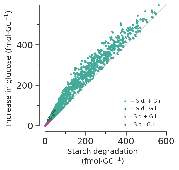

def glucose_vs_starch_subfig(ax):
    x = [0, 600]
    y = [0, 600]

    size = 10

    ax.plot(x, y, c="grey", alpha=0.5, clip_on=False, linewidth=1)

    conditions = [
        sucrose_deg_and_glc_import,
        no_sucrose_deg_glc_import,
        no_sucrose_deg_no_glc_import,
        sucrose_deg_no_glc_import,
    ]
    colours = [
        sns.color_palette()[2],
        sns.color_palette()[3],
        sns.color_palette()[4],
        sns.color_palette()[8],
    ]
    labels = ["+ Suc deg + Glc import", "- Suc deg + Glc import", "- Suc deg - Glc import", "+ Suc deg - Glc import"]

    glucose_increase_max = glc_increase_per_gc.max()

    for condition, colour, label in zip(conditions, colours, labels):
        ax.scatter(
            starch_per_gc[starch > 0][condition],
            glc_increase_per_gc[starch > 0][condition],
            color=colour,
            s=size,
            label=label,
            linewidths=0,
            clip_on=False,
        )

    ax.set_xlabel("Starch degradation\n" r"(fmol$\cdot$GC$^{-1}$)", size="medium")
    ax.set_ylabel("Increase in glucose (fmol$\cdot$GC$^{-1}$)", size="medium")

    #y_max = glucose_increase_max
    y_max = 600
    x_max = 600
    major_increment = 200
    ax.set_ylim(None, y_max)
    ax.set_xlim(None, x_max)
    ax.spines["left"].set_bounds(0, y_max)
    ax.spines["bottom"].set_bounds(0, x_max)
    ax.xaxis.set_major_locator(MultipleLocator(major_increment))
    ax.xaxis.set_minor_locator(AutoMinorLocator(2))
    ax.yaxis.set_major_locator(MultipleLocator(major_increment))
    ax.yaxis.set_minor_locator(AutoMinorLocator(2))
    ax.set_aspect("equal")

#     ax.vlines(
#         184, ymin=0, ymax=570, linewidth=1, linestyle="--", color=sns.color_palette()[6]
#     )
#     ax.text(
#         184,
#         570,
#         "Horrer et al. (2016)",
#         ha="center",
#         va="bottom",
#         size="x-small",
#         color=sns.color_palette()[6],
#     )

    ax.legend(
        loc="lower right", bbox_to_anchor=(1, 0), handletextpad=0, fontsize='x-small'
        #prop={'family': 'DejaVu Sans Mono', 'size': 'x-small'},
    )

    return ax


fig, ax = plt.subplots()

glucose_vs_starch_subfig(ax)

fig.savefig("../outputs/constraint_scan/starch_vs_glucose.svg")
fig.savefig("../outputs/constraint_scan/starch_vs_glucose.png", dpi=300)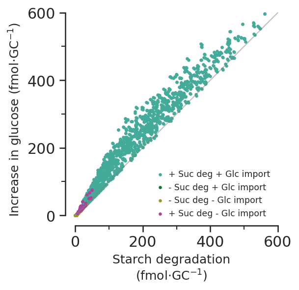

Combine subfigures

fig, axs = plt.subplots(2, 2, figsize=(10, 10))

plt.subplots_adjust(hspace=0.5, wspace=0.35)

phloemoutput_subfig(axs[0][0])

photons_vs_carbon_export_subfig(axs[0][1])

starch_vs_os_subfig(axs[1][0])

glucose_vs_starch_subfig(axs[1][1])
axs[1][1].get_legend().remove()

for ax, letter in zip(
    [axs[0][0], axs[0][1], axs[1][0], axs[1][1]], ["A", "B", "C", "D"]
):
    if letter != "D":
        ax.text(-0.4, 1.06, letter, transform=ax.transAxes, size=20, weight="bold")
    else:
        ax.text(-0.333, 1.06, letter, transform=ax.transAxes, size=20, weight="bold")

fig.savefig(
    "../outputs/constraint_scan/constraint_scan_analysis_plot.svg", transparent=True
)
fig.savefig(
    "../outputs/constraint_scan/constraint_scan_analysis_plot.png", transparent=True
)

---

Extra analyses not included

What is the ratio of mitochondrial to plastidic ATP synthase?

fig, axs = plt.subplots(1, 2, figsize=(10, 4))

axs[0].hist(
    scan_results.Plastidial_ATP_Synthase_p_gc_2[scan_constraints.light == "white"]
    / scan_results.Mitochondrial_ATP_Synthase_m_gc_2[scan_constraints.light == "white"],
    bins=100,
)
axs[0].set_title("Opening in white light")
axs[0].set_xlabel("Plastidial ATP Synthase\nMitochondrial ATP Synthase")
axs[1].hist(
    scan_results.Plastidial_ATP_Synthase_p_gc_3
    / scan_results.Mitochondrial_ATP_Synthase_m_gc_3,
    bins=100,
)
axs[1].set_title("Day in both light types")
axs[1].set_xlabel("Plastidial ATP Synthase\nMitochondrial ATP Synthase")

Text(0.5, 0, 'Plastidial ATP Synthase\nMitochondrial ATP Synthase')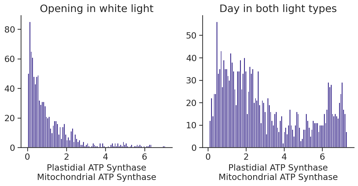

fig, ax = plt.subplots(1, figsize=(5, 4))

plastidial_atp_max = scan_results.loc[
    :, ["Plastidial_ATP_Synthase_p_gc_3", "Plastidial_ATP_Synthase_p_gc_2"]
].max(axis=1)
mitochondial_atp_max = scan_results.loc[
    :, ["Mitochondrial_ATP_Synthase_m_gc_3", "Mitochondrial_ATP_Synthase_m_gc_2"]
].max(axis=1)

for light in ["blue", "white"]:
    ax.hist(
        plastidial_atp_max[scan_constraints.light == light]
        / mitochondial_atp_max[scan_constraints.light == light],
        histtype="step",
        label=light,
    )

ax.set_xlabel("Max plastidial ATP Synthase\nMax mitochondrial ATP Synthase")

ax.legend()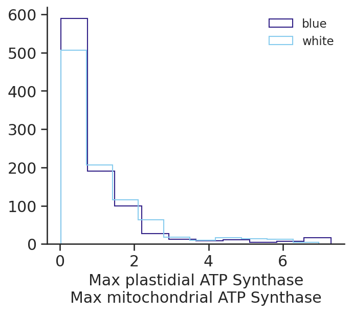

fig, ax = plt.subplots()

ax.plot([0, 0.3], [0, 0.3], c="grey", zorder=0)
ax.scatter(plastidial_atp_max, mitochondial_atp_max, s=1)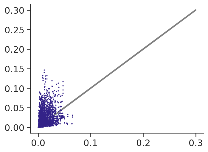

(plastidial_atp_max / mitochondial_atp_max).min()

0.016260605303926066

Almost all starch is used for glucose, and PEP carboxykinase reaction never runs

(scan_results.PEPCARBOX_RXN_c_gc_2 > 0).sum()

77

(scan_results.PEPDEPHOS_RXN_c_gc_2 > 0).sum()

1237

((scan_results.MALTODEG_RXN_c_gc_2 > 0) & (scan_results.PEPDEPHOS_RXN_c_gc_2 > 0)).sum()

1227

((scan_results.MALTODEG_RXN_c_gc_2 > 0) & (scan_results.PYRUVDEH_RXN_m_gc_2 > 0)).sum()

1227

(
    (scan_results.MALTODEG_RXN_c_gc_2 > 0)
    & (scan_results.ISOCITRATE_DEHYDROGENASE_NAD_RXN_m_gc_2 > 0)
).sum()

1266

(
    scan_results[(scan_results.MALTODEG_RXN_c_gc_2 > 0)].MALTODEG_RXN_c_gc_2 / 2
    - scan_results[(scan_results.MALTODEG_RXN_c_gc_2 > 0)].PEPDEPHOS_RXN_c_gc_2
).hist(bins=100)

(
    scan_results[(scan_results.MALTODEG_RXN_c_gc_2 > 0)].MALTODEG_RXN_c_gc_2 / 2
    - scan_results[(scan_results.MALTODEG_RXN_c_gc_2 > 0)].PYRUVDEH_RXN_m_gc_2
).hist(bins=100)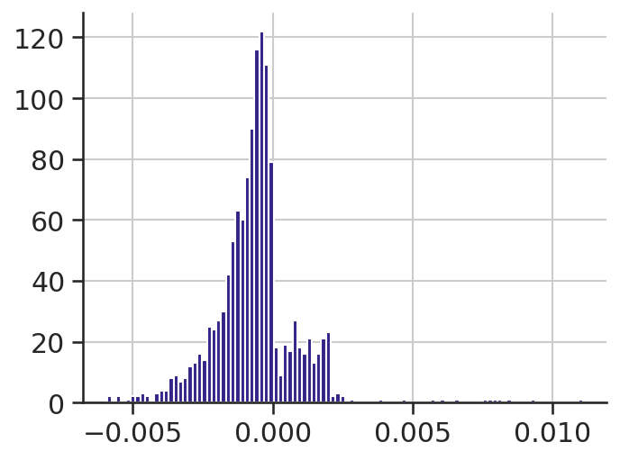

(
    scan_results[(scan_results.MALTODEG_RXN_c_gc_2 > 0)].MALTODEG_RXN_c_gc_2
    - scan_results[
        (scan_results.MALTODEG_RXN_c_gc_2 > 0)
    ].ISOCITRATE_DEHYDROGENASE_NAD_RXN_m_gc_2
)

0       0.001622
1       0.005446
3       0.001043
4       0.001028
6       0.006612
          ...   
1931    0.003674
1932    0.002604
1933    0.007325
1934    0.002005
1935    0.005452
Length: 1266, dtype: float64

(scan_results.MAL_total_pseudolinker_2 > 0).sum()

433

scan_constraints[
    (
        (scan_results.MAL_total_pseudolinker_2 - scan_results.MAL_total_pseudolinker_1)
        > 0
    )
]

	P_abs	T_l	A_l	V_gc_ind	FqFm	R_ch	R_ch_vol	L_air	L_epidermis	Vac_frac	...	N_gcs	n	m	r	s	C_apo	A_closed	A_open	ATPase	light
1	0.923180	0.000190	1.0	1.250880e-12	0.889162	0.093534	0.195869	0.337197	0.196606	0.837767	...	1.064044e+09	2.025073	0.946228	5.400144e-14	1.664063e-13	0.023524	2.500598	9.754649	0.549826	white
6	0.912552	0.000236	1.0	2.797833e-12	0.791717	0.122612	0.211564	0.203218	0.121087	0.788955	...	8.580407e+08	1.718809	0.985739	6.484944e-14	2.811758e-13	0.028334	1.156307	11.339261	2.620532	white
7	0.811951	0.000203	1.0	1.725438e-12	0.862305	0.134778	0.202345	0.342059	0.149051	0.886573	...	5.641395e+08	2.345712	0.922066	7.661761e-14	1.713217e-13	0.024734	3.836327	11.685743	0.807819	white
13	0.868580	0.000235	1.0	2.230336e-12	0.813387	0.143595	0.210389	0.231901	0.233709	0.788520	...	8.827028e+08	1.563814	0.955703	5.755866e-14	2.976694e-13	0.032311	2.576765	10.693166	4.401374	white
28	0.905738	0.000226	1.0	2.077161e-12	0.858599	0.065746	0.199877	0.232093	0.200455	0.892994	...	1.832267e+08	2.259343	0.879945	6.486503e-14	1.705626e-13	0.027999	2.573815	6.189742	0.199106	white
...	...	...	...	...	...	...	...	...	...	...	...	...	...	...	...	...	...	...	...	...	...
1929	0.963328	0.000213	1.0	3.549447e-12	0.822882	0.088125	0.207902	0.284514	0.172490	0.882110	...	3.941232e+08	1.836419	0.800060	7.761785e-14	1.283119e-13	0.025384	3.250332	8.157482	5.580050	blue
1930	0.878002	0.000222	1.0	2.235053e-12	0.861774	0.132702	0.209615	0.209708	0.145820	0.865507	...	3.784323e+08	2.348202	0.814245	5.768938e-14	2.320267e-13	0.030561	2.664441	11.247607	3.675367	blue
1932	0.957473	0.000185	1.0	2.755496e-12	0.798181	0.097823	0.201847	0.193194	0.138359	0.823731	...	6.623405e+08	1.889247	0.969003	6.787495e-14	1.566538e-13	0.032169	1.321999	5.766979	2.750124	blue
1933	0.816118	0.000174	1.0	2.957736e-12	0.825422	0.149150	0.200244	0.323872	0.209562	0.830375	...	9.035571e+08	1.971395	0.971101	7.917051e-14	2.960270e-13	0.031594	1.293918	7.247967	1.492903	blue
1935	0.953724	0.000240	1.0	1.884973e-12	0.894087	0.135577	0.189014	0.241198	0.137301	0.844829	...	5.504971e+08	1.561648	0.977668	6.731378e-14	2.085531e-13	0.036108	2.326208	9.325369	4.832752	blue

375 rows × 22 columns

#starch[1384]

#(scan_constraints.loc[1384] - scan_constraints.mean()) / scan_constraints.std()

#scan_constraints.loc[1384].ATPase

scan_constraints.mean().ATPase

/tmp/ipykernel_8731/856568451.py:1: FutureWarning: The default value of numeric_only in DataFrame.mean is deprecated. In a future version, it will default to False. In addition, specifying 'numeric_only=None' is deprecated. Select only valid columns or specify the value of numeric_only to silence this warning.
  scan_constraints.mean().ATPase

8.53114718372621

#atpase_constrained[1384]

#scan_results.loc[1384].MALTODEG_RXN_c_gc_2 / starch[1384] * 100

#scan_results.loc[1384].RXN_2141_p_gc_2

#scan_results.loc[1384].MALATE_DEH_RXN_m_gc_2

#scan_results.loc[1384].ISOCITRATE_DEHYDROGENASE_NAD_RXN_m_gc_2

#(scan_gc_constraints.loc[1384] - scan_gc_constraints.mean()) / scan_gc_constraints.std()

for i in [i+1 for i in range(4)]:
    reaction = f"PALMITATE_c_gc_Linker_{i}"
    print(reaction)
    print(scan_results.loc[:, reaction].sum())

PALMITATE_c_gc_Linker_1
0.0
PALMITATE_c_gc_Linker_2
0.0
PALMITATE_c_gc_Linker_3
0.0
PALMITATE_c_gc_Linker_4
0.0

scan_results.filter(like="ATPase", axis=1)

	PROTON_ATPase_c_me_1	PROTON_ATPase_c_me_2	PROTON_ATPase_c_me_3	PROTON_ATPase_c_me_4	PROTON_ATPase_c_gc_1	PROTON_ATPase_c_gc_2	PROTON_ATPase_c_gc_3	PROTON_ATPase_c_gc_4	ATPase_tx_me_1	ATPase_tx_me_2	ATPase_tx_me_3	ATPase_tx_me_4	ATPase_tx_gc_1	ATPase_tx_gc_2	ATPase_tx_gc_3	ATPase_tx_gc_4
0	1.107532	3.646232	3.763789	1.104726	0.000025	0.004851	0.004851	0.000025	10.025916	12.182122	12.182122	10.025916	0.000444	0.000973	0.000973	0.000444
1	1.271757	4.186898	4.311376	1.268535	0.000057	0.000585	0.000585	0.000057	10.025916	12.468127	12.468127	10.025916	0.000444	0.000967	0.000967	0.000444
2	1.131079	3.723755	3.832643	1.128600	0.000000	0.004505	0.000000	0.000000	10.025916	12.223283	12.223283	10.025916	0.000444	0.000598	0.000598	0.000444
3	1.207758	3.976199	4.097909	1.204698	0.000583	0.004855	0.002277	0.000583	10.025916	12.356973	12.356973	10.025916	0.000444	0.000508	0.000508	0.000444
4	1.260299	4.149174	4.286096	1.257106	0.000025	0.011479	0.007823	0.000025	10.025916	12.448415	12.448415	10.025916	0.000444	0.000614	0.000614	0.000444
...	...	...	...	...	...	...	...	...	...	...	...	...	...	...	...	...
1931	1.105102	3.315307	3.773362	1.102419	0.000025	0.006605	0.006605	0.000025	10.025916	10.025916	12.273932	10.025916	0.000444	0.000444	0.001019	0.000444
1932	1.261907	3.785721	4.297397	1.258843	0.000057	0.001822	0.001822	0.000057	10.025916	10.025916	12.558822	10.025916	0.000444	0.000444	0.001011	0.000444
1933	1.056017	3.168052	3.599472	1.053454	0.000057	0.001349	0.001349	0.000057	10.025916	10.025916	12.183832	10.025916	0.000444	0.000444	0.001976	0.000444
1934	1.228512	3.685537	4.184889	1.225530	0.000025	0.003092	0.003092	0.000215	10.025916	10.025916	12.498539	10.025916	0.000444	0.000444	0.000641	0.000444
1935	1.256399	3.769198	4.279254	1.253349	0.000057	0.002660	0.002660	0.000057	10.025916	10.025916	12.549088	10.025916	0.000444	0.000444	0.000826	0.000444

1934 rows × 16 columns

scan_constraints

	P_abs	T_l	A_l	V_gc_ind	FqFm	R_ch	R_ch_vol	L_air	L_epidermis	Vac_frac	...	N_gcs	n	m	r	s	C_apo	A_closed	A_open	ATPase	light
0	0.815093	0.000194	1.0	2.262641e-12	0.809297	0.179970	0.191527	0.240879	0.214860	0.858645	...	4.484392e+08	1.933548	0.992641	7.886553e-14	1.678654e-13	0.033679	2.321339	11.318979	10.816668	white
1	0.923180	0.000190	1.0	1.250880e-12	0.889162	0.093534	0.195869	0.337197	0.196606	0.837767	...	1.064044e+09	2.025073	0.946228	5.400144e-14	1.664063e-13	0.023524	2.500598	9.754649	0.549826	white
2	0.830507	0.000220	1.0	5.035745e-13	0.821060	0.167889	0.204824	0.331556	0.205674	0.816618	...	5.758277e+08	2.141889	0.972835	6.579620e-14	2.457118e-13	0.034062	2.802180	3.338120	7.823891	white
3	0.880998	0.000192	1.0	8.629192e-13	0.866582	0.051244	0.204472	0.309538	0.169957	0.813726	...	3.851195e+08	2.077401	0.940848	5.747590e-14	1.515328e-13	0.029770	3.399462	9.936390	12.606738	white
4	0.915597	0.000220	1.0	7.391447e-13	0.846358	0.059969	0.193449	0.352066	0.238671	0.810491	...	1.046353e+09	2.396012	0.817798	7.654181e-14	1.652973e-13	0.028420	3.305233	7.650706	10.970481	white
...	...	...	...	...	...	...	...	...	...	...	...	...	...	...	...	...	...	...	...	...	...
1931	0.849808	0.000174	1.0	2.640313e-12	0.880585	0.134355	0.193583	0.289995	0.213762	0.794641	...	4.117855e+08	1.711337	0.981658	6.898412e-14	1.062431e-13	0.033170	1.843784	11.521533	16.039577	blue
1932	0.957473	0.000185	1.0	2.755496e-12	0.798181	0.097823	0.201847	0.193194	0.138359	0.823731	...	6.623405e+08	1.889247	0.969003	6.787495e-14	1.566538e-13	0.032169	1.321999	5.766979	2.750124	blue
1933	0.816118	0.000174	1.0	2.957736e-12	0.825422	0.149150	0.200244	0.323872	0.209562	0.830375	...	9.035571e+08	1.971395	0.971101	7.917051e-14	2.960270e-13	0.031594	1.293918	7.247967	1.492903	blue
1934	0.934550	0.000234	1.0	1.122269e-12	0.799613	0.047919	0.202674	0.351210	0.192651	0.814861	...	1.121745e+09	2.313188	0.857276	6.322405e-14	1.450759e-13	0.023108	2.345988	6.138390	2.756515	blue
1935	0.953724	0.000240	1.0	1.884973e-12	0.894087	0.135577	0.189014	0.241198	0.137301	0.844829	...	5.504971e+08	1.561648	0.977668	6.731378e-14	2.085531e-13	0.036108	2.326208	9.325369	4.832752	blue

1934 rows × 22 columns

print(min(scan_constraints.P_abs))
print(min(scan_results.Phloem_tx_overall))

0.8101673308967071
12.675979574938289

print(max(scan_constraints.R_ch_vol))
print(min(scan_constraints.R_ch_vol))

0.2128525606703812
0.1889727321710271